Visualising your fitted non-linear dimension reduction model in the high-dimensional data space

Jayani P.G. Lakshika

Joint work with Prof. Dianne Cook, Dr. Paul Harrison, Dr. Michael Lydeamore, Dr. Thiyanga S. Talagala

quollr

questioning how a high-dimensional object looks in low-dimensions using r

Motivation

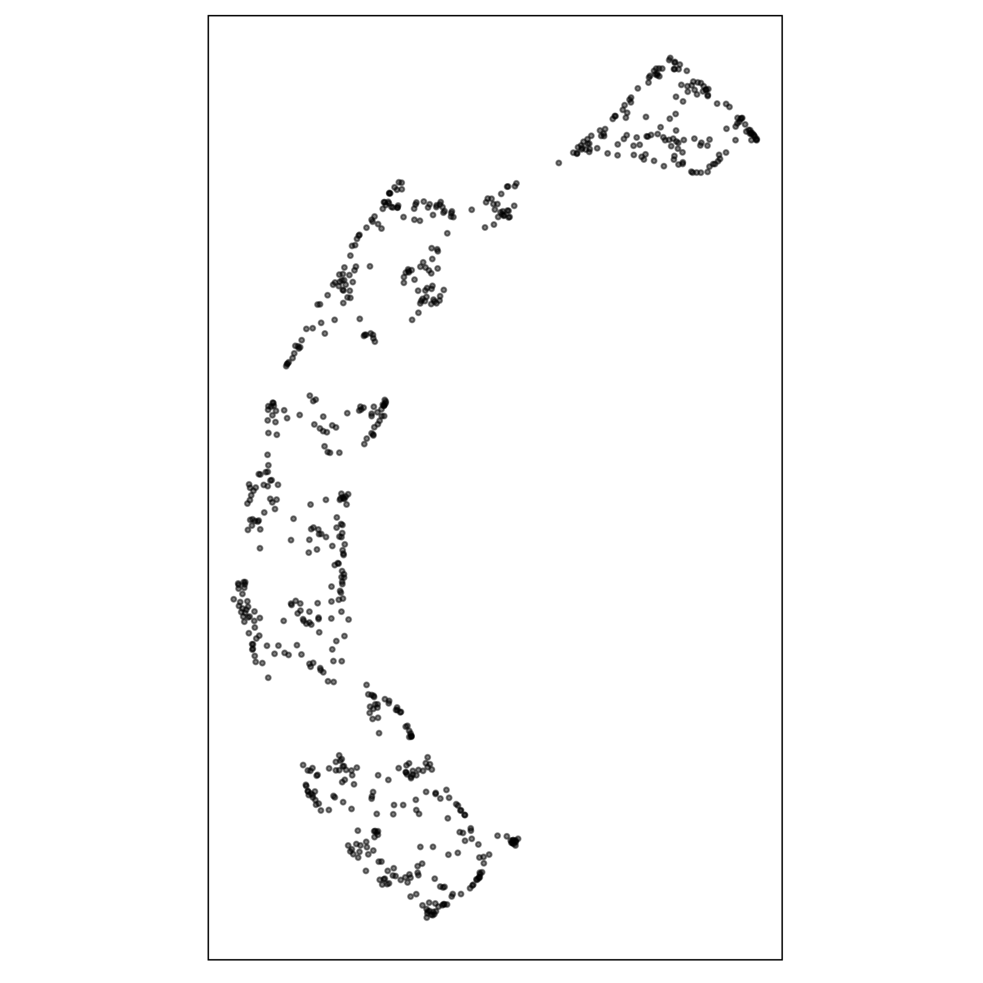
Single-cell gene expression: same data, different NLDR + hyper-parameters

How do you decide which is the best representation?

This is the published figure.

Here is the 9D data viewed using a grand tour, linear projections into 2D.

Software: langevitour

Show “model-in-the-data-space”

data-in-the-model-space

model-in-the-data-space

Start with a simple example: S-curve in 7D

data-in-the-model-space

model-in-the-data-space

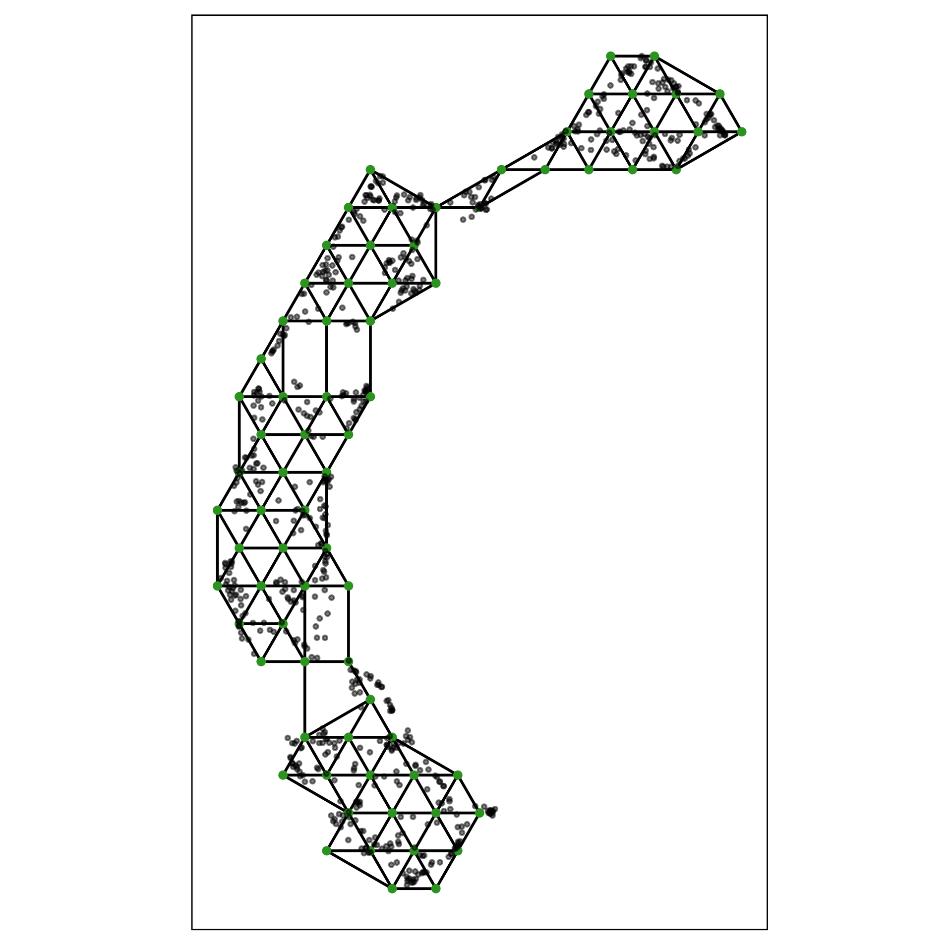
Overview of method

1. Construct the \(2\text{-}D\) model

2. Lift the model into high-dimensions

Steps of the algorithm

1. Construct the \(2\text{-}D\) model

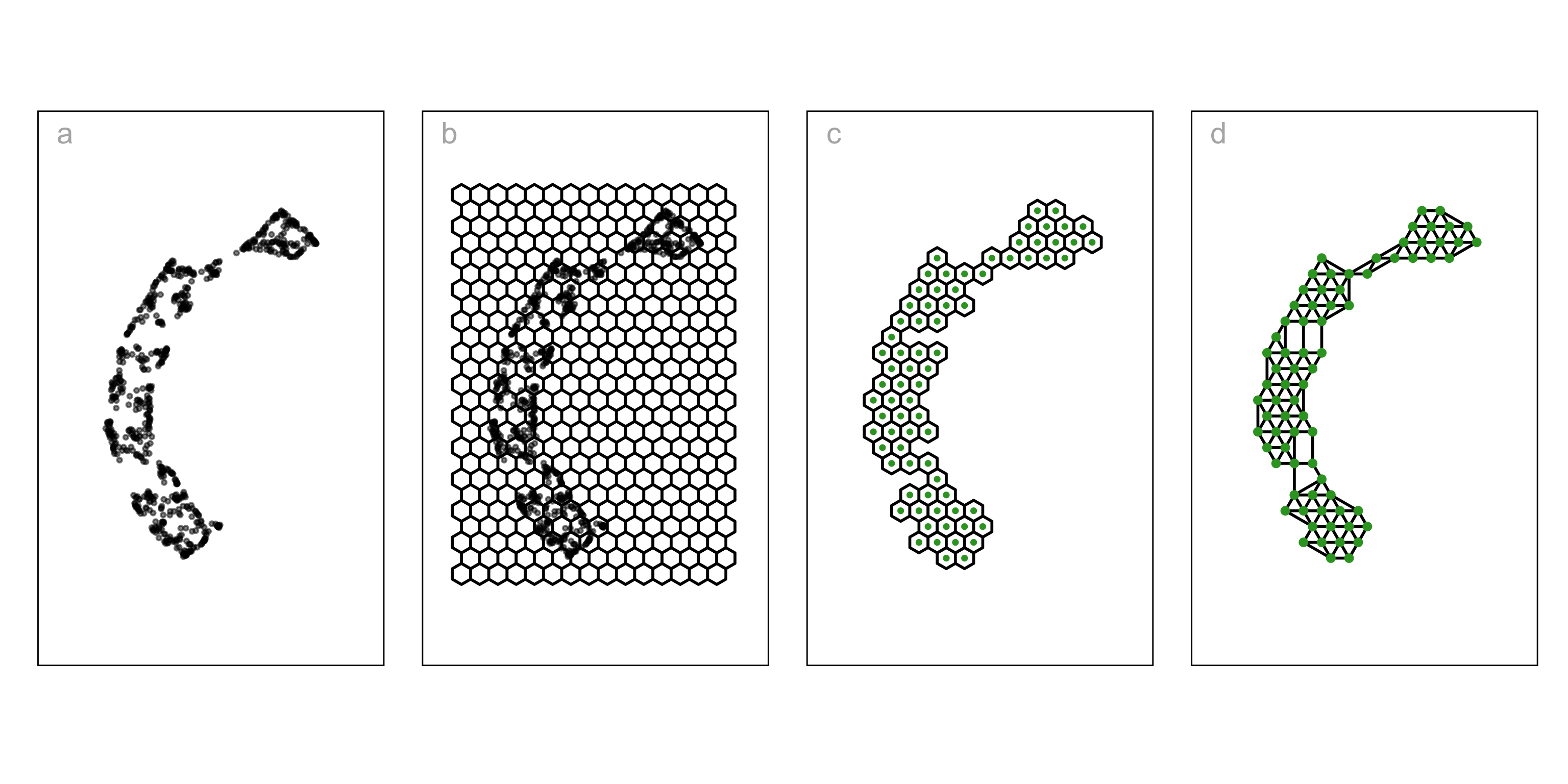
1. NLDR layout, b. hex bin (hex_binning() and geom_hexgrid()), c. bin centers (extract_hexbin_centroids()), d. triangulation wire frame (tri_bin_centroids(), gen_edges() and geom_trimesh()).

Steps of the algorithm

2. Lift the model into high-dimensions

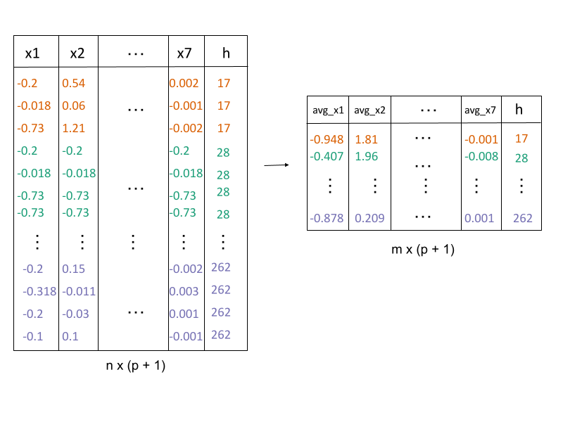
avg_highd_data()

show_langevitour()

Factors for fitting and measuring fit

• NLDR layout, different methods and different hyper-parameters
• Number of bins
• Bin start position
• Low density removal (find_low_dens_hex())
• Long edge removal (find_lg_benchmark())

• MSE in high-dimensions: mean sum of squared differences between observed and fitted values (glance())

\[\frac{1}{n}\sum_{h = 1}^{b}\sum_{i = 1}^{n_h}\sum_{j = 1}^{p} ({x}_{hij} - C^{(p)}_{hj})^2\] \(n =\) the number of observations,

\(b =\) the number of bins,

\(n_h =\) the number of observations in \(h^{th}\) bin,

\(p =\) the number of variables,

\({x}_{hij} =\) the \(j^{th}\) dimensional data of \(i^{th}\) observation in \(h^{th}\) hexagon.

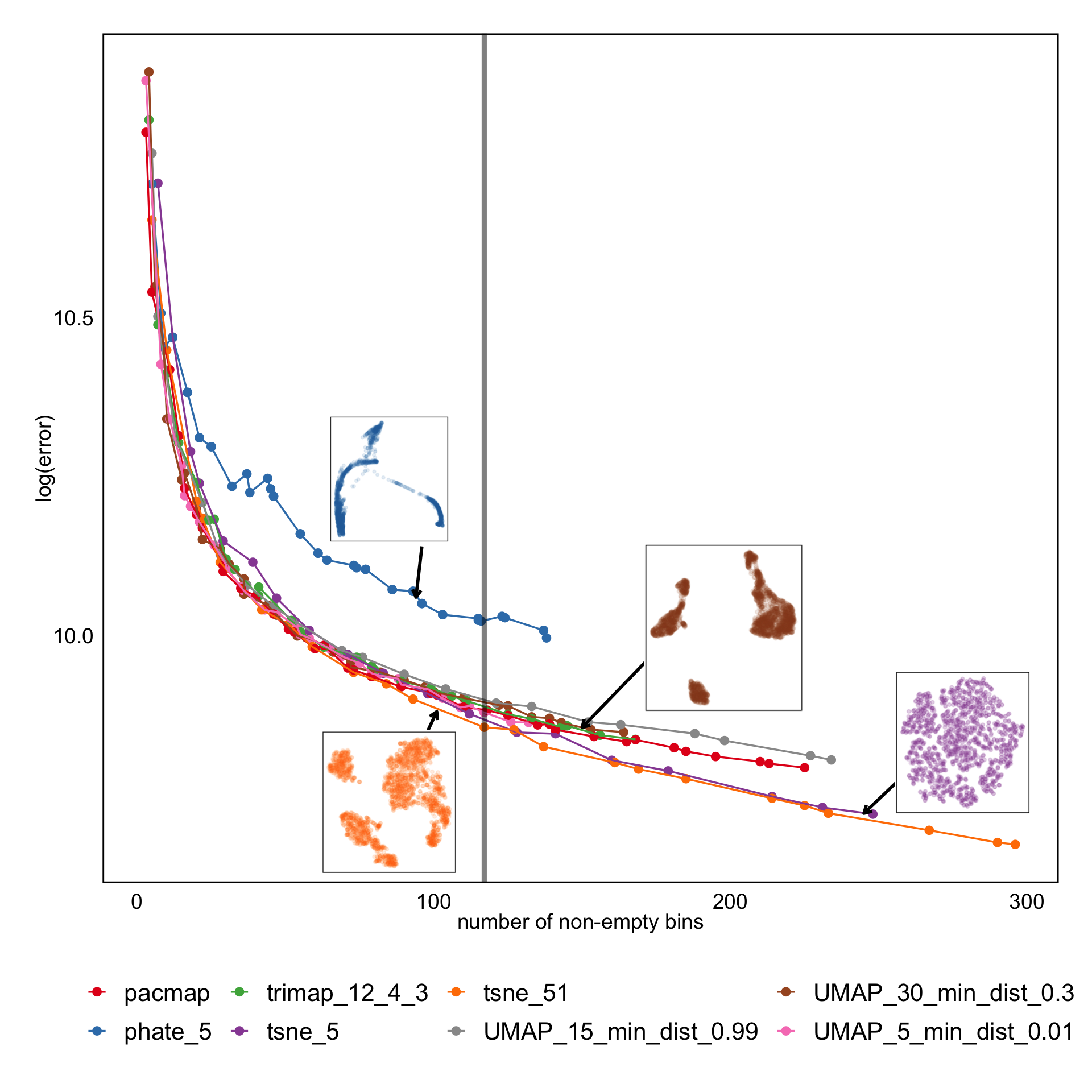
Candidates for NLDR layout

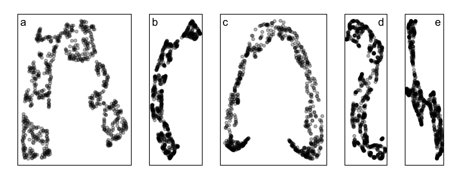
1. tSNE, b. UMAP, c. PHATE, d. TriMAP, e. PaCMAP

MSE of candidates

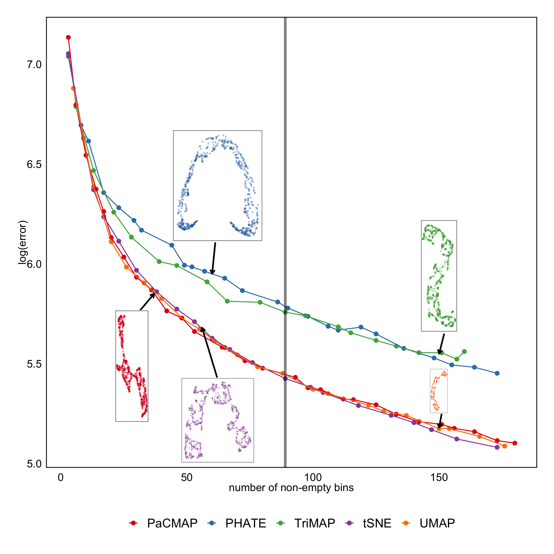
• PHATE, TriMAP not competitive
• Not much difference between any other method based on MSE
• No elbow, just gradual decrease as number of (non-empty) bins increase

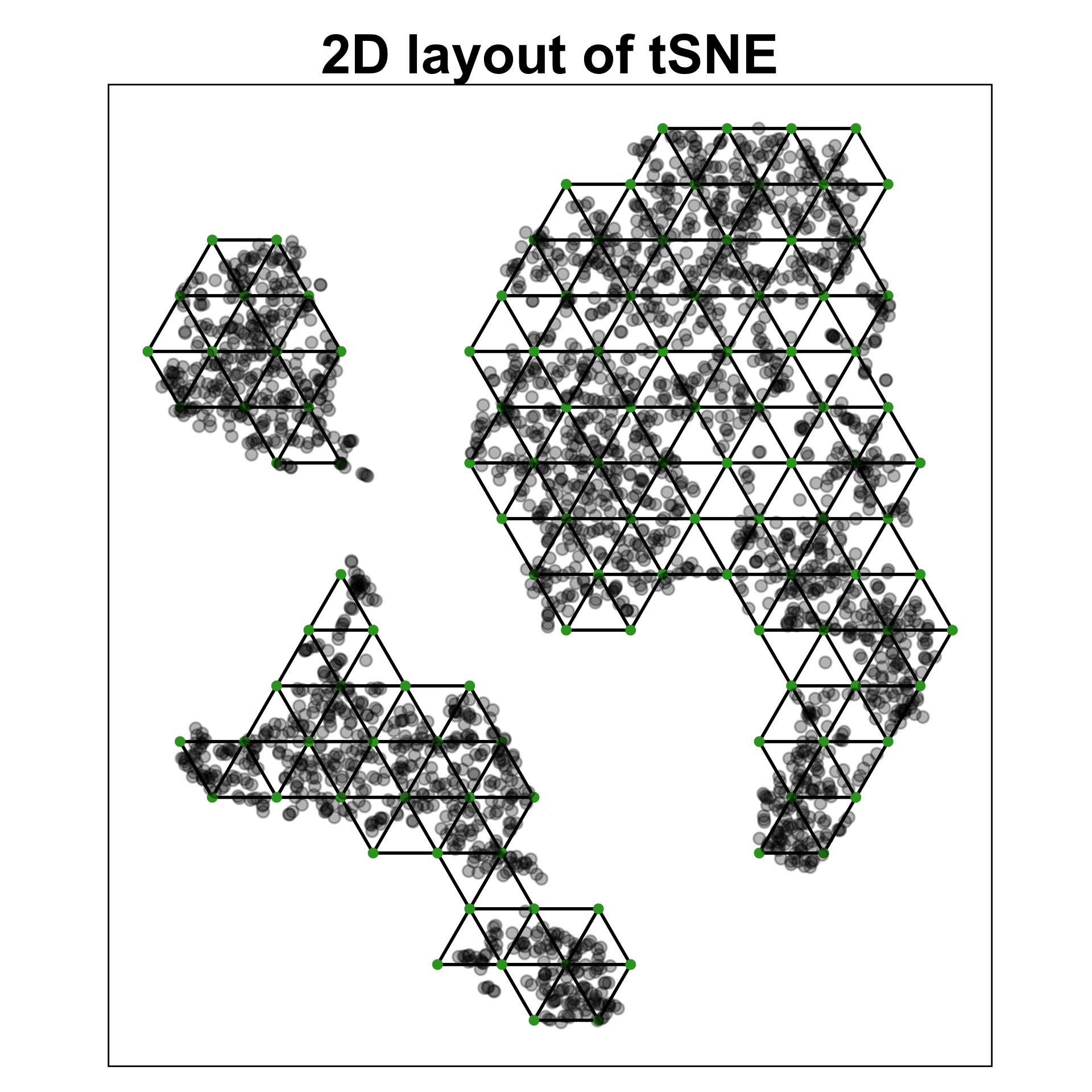
Best fit for S-curve

tSNE with perplexity: 27

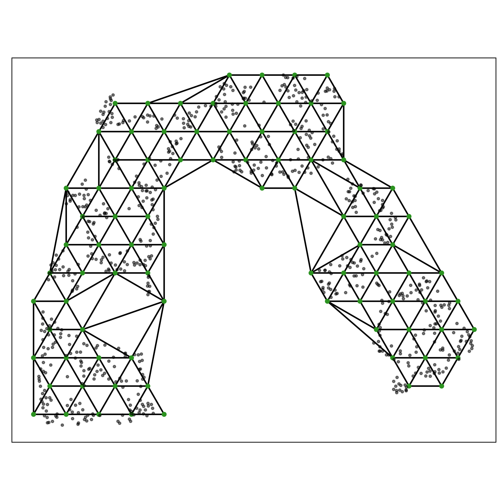
Pretty good! Can you see the twist??

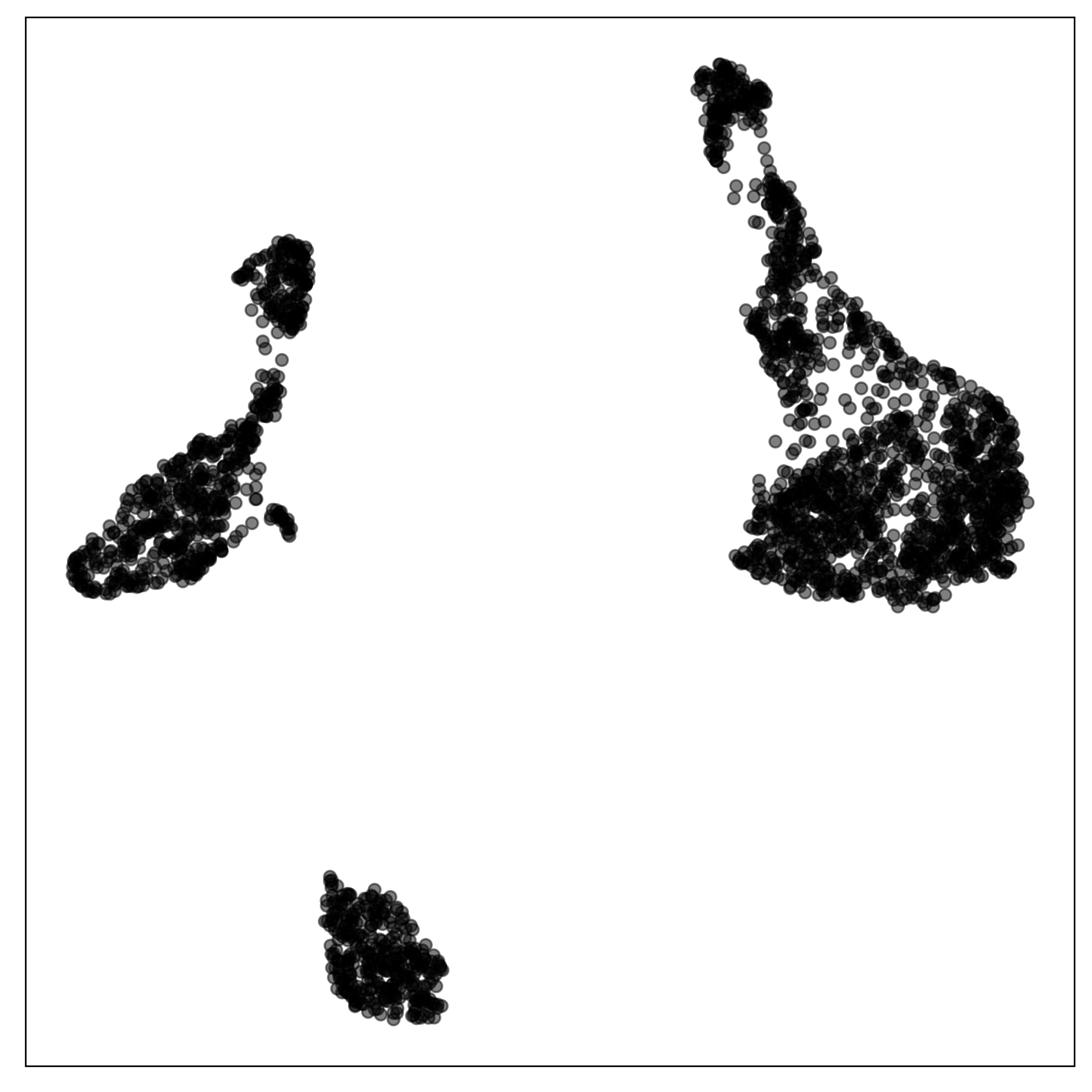
PBMC data set

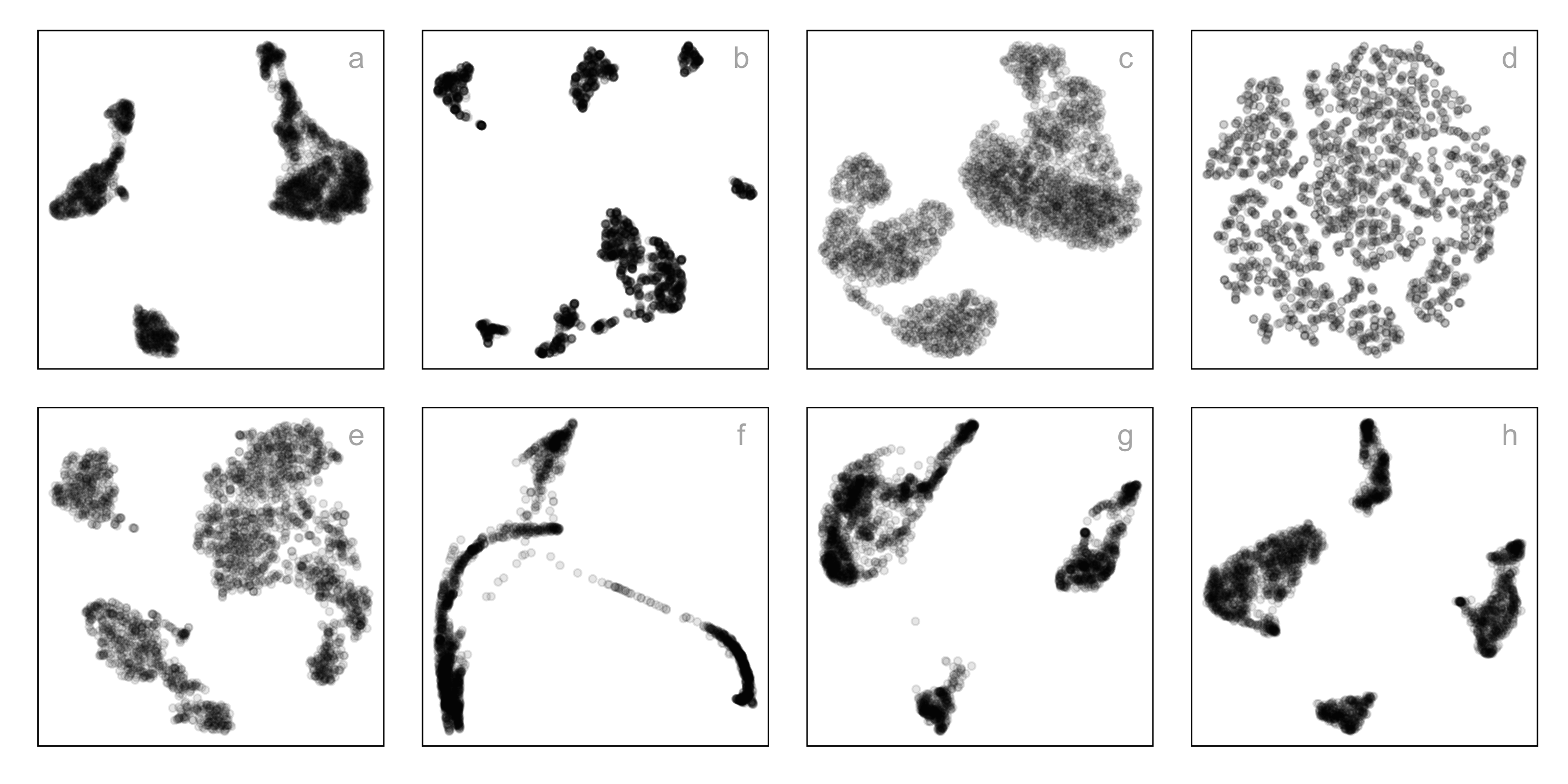
Best fit for PBMC data set

tSNE with perplexity: 30

Summary

Note

• Provided a method to create a model from a NLDR layout that can be displayed with the data to assess the fit.

• Make it easier for researchers to make better decisions on which NLDR layout is best for their work.

• It has the additional benefit that for any method you can now provide predictions for new data, of where these points will be positioned in the NLDR.

Jayani P.G. Lakshika

Collaborators: Prof. Dianne Cook, Dr. Paul Harrison, Dr. Michael Lydeamore, Dr. Thiyanga S. Talagala